Published on

Peak fitting XRD data with Python

13 min read
Authors

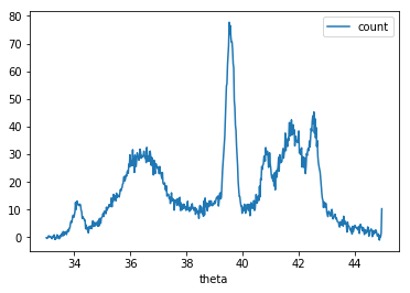
While it may not be apparent on my blog, I am graduate student studying computational material science. Our group studies the fundamental physics behind ion beam modification and radiation resistant nuclear materials. One of the techniques our experimentalists use regularly is x-ray diffraction (XRD). XRD is a technique where you point an x-ray beam at a material in a set angle and observe the resulting angles and intensities of the diffracted beam. These patterns when measures with a camera along all angles θ\theta result in peaks. The figure below shows an example pattern of ours.

XRD experimental pattern

It turns out that all XRD profiles are a combination of gaussians, lorentzians, and voigt functions. As a material scientist I had always been told that fitting is hard. But the mathematician side of me never believed it! There are numerous commercially available and open source softwares to do this job such as Origin Pro Peak Fitting, IGOR Pro, GSAS, and many others. But to me they all have one problem. They obscure the simple mathematics taking place behind the scenes. Infact in this post I will show how with numpy and scipy alone we can create our own peak fitting software that is just as successful. Later we will use the excellent python package lmfit which automates all the tedious parts of writting our own fitting software. First lets import everything we will need.

import os
import math
import random

import numpy as np
import pandas as pd
import matplotlib.pyplot as plt
from scipy import optimize, signal

from lmfit import models

# ignore used to produce images for blog
image_dir = "images"
def plot_to_blog(fig, figure_name):
    filename = os.path.expanduser(f'{image_dir}/{figure_name}')
    fig.savefig(filename)
    return filename

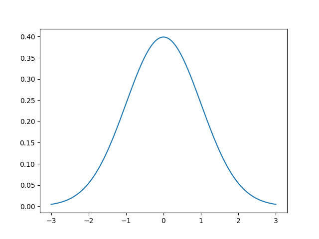
Now I promise we will get to fitting this XRD profile but first we must show what is involved in fitting gaussians, lorentzians, and voigt functions. In general this fitting process can be written as non-linear optimization where we are taking a sum of functions to reproduce the data. The gaussian function is also known as a normal distribution. In the figure below we show a gaussian with amplitude 1, mean 0, and variance 1.

f(x;A,μ,σ)=Aσ2πe[(xμ)2/2σ2]f(x; A, \mu, \sigma) = \frac{A}{\sigma\sqrt{2\pi}} e^{[{-{(x-\mu)^2}/{{2\sigma}^2}}]}

def g(x, A, μ, σ):
    return A / (σ * math.sqrt(2 * math.pi)) * np.exp(-(x-μ)**2 / (2*σ**2))

x = np.linspace(-3, 3, 1000)
fig, ax = plt.subplots()
ax.plot(x, g(x, 1, 0, 1))
plot_to_blog(fig, 'xrd-fitting-gaussian.png')
XRD Fitting Gaussian

Now I will show simple optimization using scipy which we will use for solving for this non-linear sum of functions. There is a really nice scipy.optimize.minimize method that has several optimizers. I will only use the default one for these demonstrations. Let's see this method in action. Suppose we have an unknown function plotted bellow.

def f(x):
    return np.exp(-(x-2)**2) + np.exp(-(x-6)**2/10) + 1/(x**2 + 1)

x = np.linspace(-2, 10, 1000)
fig, ax = plt.subplots()
ax.plot(x, -f(x))
plot_to_blog(fig, 'xrd-fitting-unknown.png')
XRD Fitting Unknown

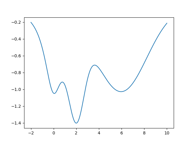
Now we will use scipy.optimize.minimize to find the global minimum of the function.

print('|{:>16}|{:>16}|{:>16}|'.format('initial','iterations','minimum'))
initial_guess = -0.5
result = optimize.minimize(lambda x: -f(x), [initial_guess])
print(f'|{initial_guess:+16.1f}|{result.nit:>16}|{result.x[0]:16.3f}|')

initial_guess = -2
result = optimize.minimize(lambda x: -f(x), [initial_guess])
print(f'|{initial_guess:+16.1f}|{result.nit:>16}|{result.x[0]:16.3f}|')

initial_guess = 9
result = optimize.minimize(lambda x: -f(x), [initial_guess])
print(f'|{initial_guess:+16.1f}|{result.nit:>16}|{result.x[0]:16.3f}|')
initialiterationsminimum
-0.550.064
-2.042.001
+9.035.955

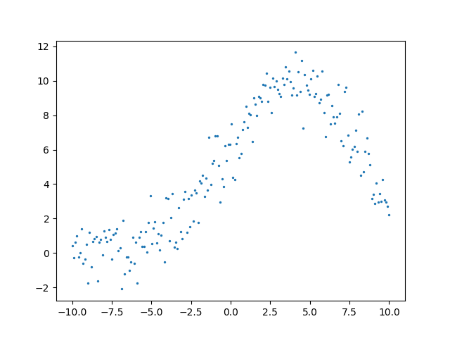
Notice how different initial guesses result in different minimums. This is true for any global optimization problem. These optimization routines do not guarantee that they have found the global minimum. A common issue we will see with fitting XRD data is that there are many of these local minimums where the routine gets stuck. This is why a good initial guess is extremely important. Let's use this optimization to fit a gaussian with some noise. See the plot below for the data we are trying to fit.

A = 100.0 # intensity
μ = 4.0  # mean
σ = 4.0 # peak width
n = 200
x = np.linspace(-10, 10, n)
y = g(x, A, μ, σ) + np.random.randn(n)

fig, ax = plt.subplots()
ax.scatter(x, y, s=2)
plot_to_blog(fig, 'xrd-fitting-gaussian-noise.png')
XRD Fitting Gaussin

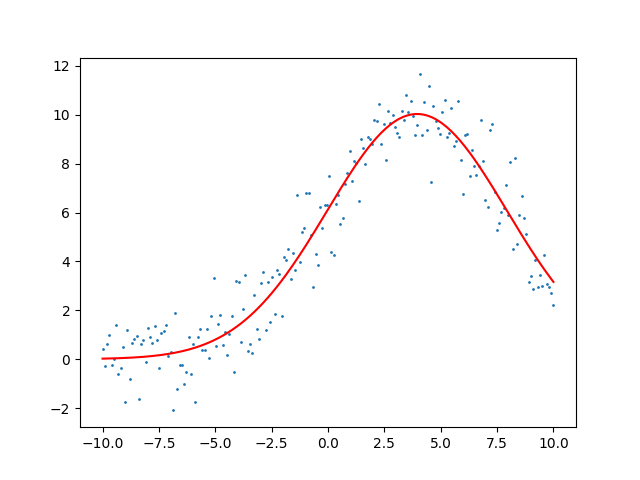
Now we will use optimization to backout what it believes the parameters of the gaussian are. In order to optimize the algorithm needs some way to measure improvement. For this we will use the mean square error as a cost function for our optimization routine.

MSE=1nn_i=1(Y_iY^_i)2MSE = \frac{1}{n} \sum^n\_{i=1} (Y\_i - \hat{Y}\_i)^2

Here Y_iY\_i and Y^_i\hat{Y}\_i represents the model values and observed values respectively. The better the fit the closer the MSE will be to zero.

def cost(parameters):
    a, b, c = parameters
    # y has been calculated in previous snippet
    return np.sum(np.power(g(x, a, b, c) - y, 2)) / len(x)

result = optimize.minimize(cost, [0, 0, 1])
print('steps', result.nit, result.fun)
print(f'amplitude: {result.x[0]:3.3f} mean: {result.x[1]:3.3f} sigma: {result.x[2]:3.3f}')
steps 15 1.0846693928147109
amplitude: 100.103 mean: 3.951 sigma: 3.980
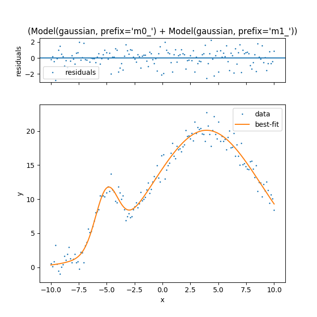
XRD Fitting Gaussin Noise OPT

That's a great fit for some simple data lets throw a harder problem at it. Let's fit two Gaussian.

g_0 = [250.0, 4.0, 5.0]
g_1 = [20.0, -5.0, 1.0]
n = 150
x = np.linspace(-10, 10, n)
y = g(x, *g_0) + g(x, *g_1) + np.random.randn(n)

fig, ax = plt.subplots()
ax.scatter(x, y, s=1)
ax.plot(x, g(x, *g_0))
ax.plot(x, g(x, *g_1))
plot_to_blog(fig, 'xrd-fitting-two-gaussian-noise.png')
XRD Fitting Gaussain Noice

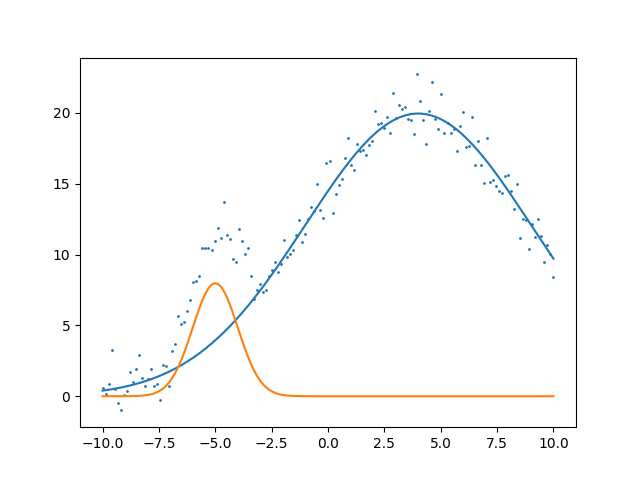
Now similarly we adapt our cost function for two gaussians and optimize. We can see that this method does exactly what we would like to do for our XRD data! I think at this point it is important to talk about our initial guess. The initial guess is very important. The computer science phrase garbage in, garbage out is extremely relevant. If you play around with the initial guess in the code below it will not always get the correct solution. This indicates that even for this problem there are many local minimums. Try setting initial_guess = np.random.randn(6) you will notice that it will get the correct solution about one out of every ten times. This is where domain knowledge comes in! Some things to know about profiles. The amplitude is always positive and never exceeds the max amplitude in the profile, the width is always positive and not extremely broad, and the mean is always between the domain. With this information we now have constraints that we can use to put bounds on our solution and initial guess. We will use this information with lmfit.

def cost(parameters):
    g_0 = parameters[:3]
    g_1 = parameters[3:6]
    return np.sum(np.power(g(x, *g_0) + g(x, *g_1) - y, 2)) / len(x)

initial_guess = [1, 0, 1, -1, 0, 1]
result = optimize.minimize(cost, initial_guess)
print('steps', result.nit, result.fun)
print(f'g_0: amplitude: {result.x[0]:3.3f} mean: {result.x[1]:3.3f} sigma: {result.x[2]:3.3f}')
print(f'g_1: amplitude: {result.x[3]:3.3f} mean: {result.x[4]:3.3f} sigma: {result.x[5]:3.3f}')
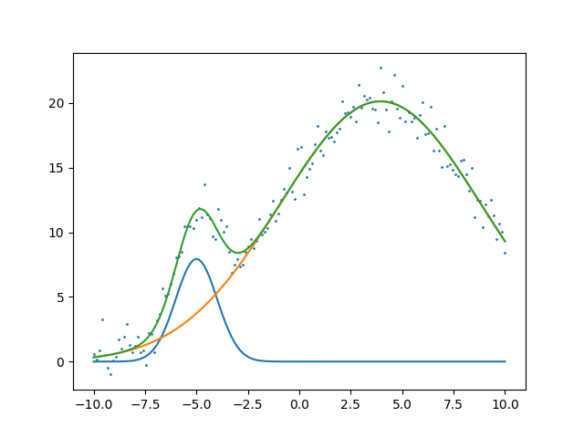
steps 71 1.0378296281115338
g_0: amplitude: 20.102 mean: -4.999 sigma: 1.010
g_1: amplitude: 245.723 mean: 3.947 sigma: 4.871

And the resulting fit shown below.

fig, ax = plt.subplots()
ax.scatter(x, y, s=1)
ax.plot(x, g(x, *result.x[:3]))
ax.plot(x, g(x, *result.x[3:6]))
ax.plot(x, g(x, *result.x[:3]) + g(x, *result.x[3:6]))
plot_to_blog(fig, 'xrd-fitting-two-gaussian-noise-opt.png')
XRD Fitting Two Gaussian Noice OPT

At this point I think it is time that we try to fit actual XRD data. We understand the method of fitting a profile. But the current method of constructing the optimization is tedious to say the least. As Raymond Hettinger always says there must be a better way! Let's use a package designed exactly for this lmfit. You can easily install it via pip install lmfit. I think of lmfit as constructing a model that represents your data by adding together several functions. In our case these functions will be the gaussians, lorentzians, and voigt. But lmfit is much more flexible than that see the available functions and you can even include your own as an arbitrary python function. Another issue that lmfit solves is mapping your function parameters to the optimization routine and adding complex constraints such as min, max, relationships between parameters, and fixed values. Interestingly I found myself constructing a similar class to their Parameter class in my code DFTFIT.

model_1 = models.GaussianModel(prefix='m1_')
model_2 = models.GaussianModel(prefix='m2_')
model = model_1 + model_2

params_1 = model_1.make_params(center=1, sigma=1)
params_2 = model_2.make_params(center=-1, sigma=1)
params = params_1.update(params_2)

output = model.fit(y, params, x=x)
fig, gridspec = output.plot(data_kws={'markersize': 1})
plot_to_blog(fig, 'xrd-fitting-two-gaussian-noise-lmfit.png')
XRD Fitting Two Gaussian Noise lmfit

Notice how lmfit made the model construction much easier. You simply add together your models and set the initial guess parameters for each through make_params. If you would like to set bounds and additional constraints use set_param_hint. Using the domain knowledge that we have about XRD we can simplify the creation of these models greatly. This will setup default initial guesses, set bounds on variable values, and allow for a python dictionary as a spec.

def generate_model(spec):
    composite_model = None
    params = None
    x = spec['x']
    y = spec['y']
    x_min = np.min(x)
    x_max = np.max(x)
    x_range = x_max - x_min
    y_max = np.max(y)
    for i, basis_func in enumerate(spec['model']):
        prefix = f'm{i}_'
        model = getattr(models, basis_func['type'])(prefix=prefix)
        if basis_func['type'] in ['GaussianModel', 'LorentzianModel', 'VoigtModel']: # for now VoigtModel has gamma constrained to sigma
            model.set_param_hint('sigma', min=1e-6, max=x_range)
            model.set_param_hint('center', min=x_min, max=x_max)
            model.set_param_hint('height', min=1e-6, max=1.1*y_max)
            model.set_param_hint('amplitude', min=1e-6)
            # default guess is horrible!! do not use guess()
            default_params = {
                prefix+'center': x_min + x_range * random.random(),
                prefix+'height': y_max * random.random(),
                prefix+'sigma': x_range * random.random()
            }
        else:
            raise NotImplemented(f'model {basis_func["type"]} not implemented yet')
        if 'help' in basis_func:  # allow override of settings in parameter
            for param, options in basis_func['help'].items():
                model.set_param_hint(param, **options)
        model_params = model.make_params(**default_params, **basis_func.get('params', {}))
        if params is None:
            params = model_params
        else:
            params.update(model_params)
        if composite_model is None:
            composite_model = model
        else:
            composite_model = composite_model + model
    return composite_model, params

Lets try the same problem that we have been working on. Again to show how there are multiple local optimums you will notice that this method does not always converge to the true solution. The spec that we have defined in the code above will work for gaussians, lorentzians, and voigt. All parameters can be initialized via params and all hints can be supplied as hints. I will show that in the final example.

spec = {
    'x': x,
    'y': y,
    'model': [
        {'type': 'GaussianModel'},
        {'type': 'GaussianModel'}
    ]
}

model, params = generate_model(spec)
output = model.fit(spec['y'], params, x=spec['x'])
fig, gridspec = output.plot(data_kws={'markersize': 1})
plot_to_blog(fig, 'xrd-fitting-two-gaussian-noise-lmfit-spec.png')
XRD Fitting Two Gaussian Noise lmfit spec

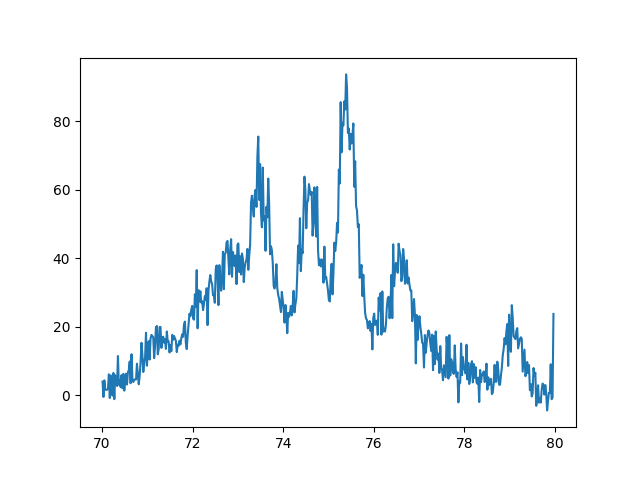
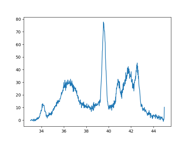
Finally here is our example XRD spectra. I will not show the actual data since my colleague would like to keep that for publication. But again here is the plot we are trying to fit. The data if from a very disordered sample due to irradiation.

XRD Fitting XRD Data

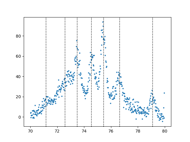
It is tedious to find all the peaks so lets write a function to help us assign initial values for guesses based on peaks. This routine uses scipy's find_peaks_cwt method. I have found it to be superior to many other peak finding algorithms out there.

def update_spec_from_peaks(spec, model_indicies, peak_widths=(10, 25), **kwargs):
    x = spec['x']
    y = spec['y']
    x_range = np.max(x) - np.min(x)
    peak_indicies = signal.find_peaks_cwt(y, peak_widths)
    np.random.shuffle(peak_indicies)
    for peak_indicie, model_indicie in zip(peak_indicies.tolist(), model_indicies):
        model = spec['model'][model_indicie]
        if model['type'] in ['GaussianModel', 'LorentzianModel', 'VoigtModel']:
            params = {
                'height': y[peak_indicie],
                'sigma': x_range / len(x) * np.min(peak_widths),
                'center': x[peak_indicie]
            }
            if 'params' in model:
                model.update(params)
            else:
                model['params'] = params
        else:
            raise NotImplemented(f'model {basis_func["type"]} not implemented yet')
    return peak_indicies

spec = {
    'x': df.index.values,
    'y': df['count'].values,
    'model': [
        {'type': 'VoigtModel'},
        {'type': 'VoigtModel'},
        {'type': 'VoigtModel'},
        {'type': 'VoigtModel'},
        {'type': 'GaussianModel'},
        {'type': 'GaussianModel'},
        {'type': 'GaussianModel'},
        {'type': 'GaussianModel'},
    ]
}

peaks_found = update_spec_from_peaks(spec, [0, 1, 2, 3, 4, 5, 6], peak_widths=(15,))
fig, ax = plt.subplots()
ax.scatter(spec['x'], spec['y'], s=4)
for i in peaks_found:
    ax.axvline(x=spec['x'][i], c='black', linestyle='dotted')

plot_to_blog(fig, 'xrd-fitting-xrd-peaks.png')
XRD Fitting xrd peaks

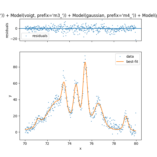
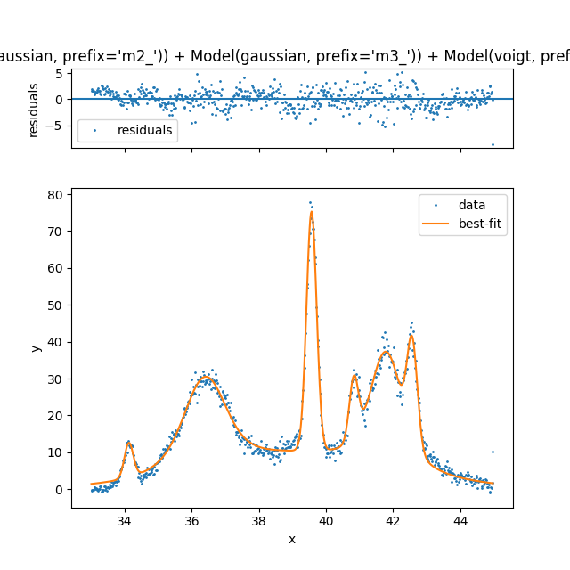
Now using are good initial guesses for the peaks we begin our optimization.

model, params = generate_model(spec)
output = model.fit(spec['y'], params, x=spec['x'])
fig, gridspec = output.plot(data_kws={'markersize':  1})
plot_to_blog(fig, 'xrd-fitting-xrd-total.png')
XRD fitting xrd total
fig, ax = plt.subplots()
ax.scatter(spec['x'], spec['y'], s=4)
components = output.eval_components(x=spec['x'])
print(len(spec['model']))
for i, model in enumerate(spec['model']):
    ax.plot(spec['x'], components[f'm{i}_'])

plot_to_blog(fig, 'xrd-fitting-xrd-components.png')
XRD fitting xrd components

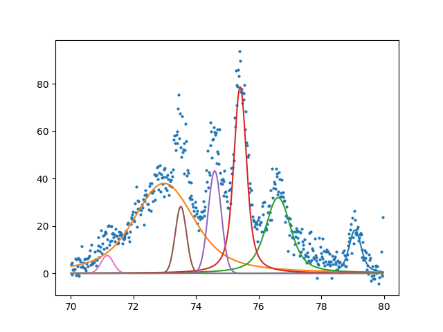
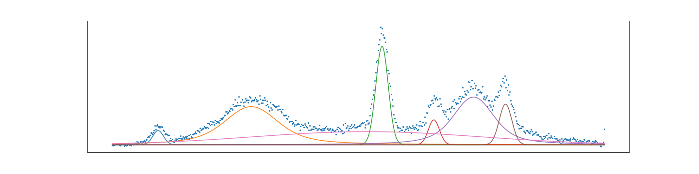
Finally showing that with a little bit of code we can automate a method for fitting that is equally impressive to commercial software. I would argue that this method is more flexible and does not hide the detail of fitting. Having a spec also makes it easy to save a model as a template for future fit. Something that I haven't seen before. To show how detailed the spec can be here is an example of fitting a profile that has hidden peaks.

XRD Fitting xrd data complex

Here is the complex spec showing off all of the features. We see that it is possible to tightly constrain the location of peaks. Something that is not easily possible in other software.

spec = {
    'x': df.index.values,
    'y': df['count'].values,
    'model': [
        {
            'type': 'GaussianModel',
            'params': {'center': 34.11, 'height': 13.08, 'sigma': 0.1},
            'help': {'center': {'min': 33.5, 'max': 34.5}}
        },
        {
            'type': 'VoigtModel',
            'params': {'center': 36.37, 'height': 30.94, 'sigma': 0.1, 'gamma': 0.1},
            'help': {'center': {'min': 35, 'max': 37}}
        },
        {'type': 'GaussianModel', 'params': {'center': 39.57, 'height': 76.56, 'sigma': 0.1}},
        {
            'type': 'GaussianModel',
            'params': {'center': 40.85, 'height': 30.77, 'sigma': 0.1},
            'help': {'center': {'min': 40, 'max': 42}}
        },
        {'type': 'VoigtModel', 'params': {'center': 41.73, 'height': 38.44, 'sigma': 0.05, 'gamma': 0.15}},
        {
            'type': 'GaussianModel',
            'params': {'center': 42.55, 'height': 45.29, 'sigma': 0.1},
            'help': {'center': {'min': 42, 'max': 43}}
        },
        {'type': 'GaussianModel', 'help': {'center': {'max': 39.2}}},
        #{'type': 'GaussianModel'},
        #{'type': 'GaussianModel'}
    ]
}

model, params = generate_model(spec)
output = model.fit(spec['y'], params, x=spec['x'])
fig, gridspec = output.plot(data_kws={'markersize': 1})
plot_to_blog(fig, 'xrd-fitting-xrd-data-complex-lmfit.png')
XRD fitting xrd data complex lmfit
fig, ax = plt.subplots()
ax.scatter(spec['x'], spec['y'], s=4)
components = output.eval_components(x=spec['x'])
print(len(spec['model']))
for i, model in enumerate(spec['model']):
    ax.plot(spec['x'], components[f'm{i}_'])

plot_to_blog(fig, 'xrd-fitting-xrd-complex-components.png')
XRD fitting xrd complex components

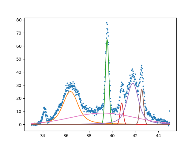
So far I have shown the fitting but we most importantly want the parameters for further analysis.

def print_best_values(spec, output):
    model_params = {
        'GaussianModel':   ['amplitude', 'sigma'],
        'LorentzianModel': ['amplitude', 'sigma'],
        'VoigtModel':      ['amplitude', 'sigma', 'gamma']
    }
    best_values = output.best_values
    print('center    model   amplitude     sigma      gamma')
    for i, model in enumerate(spec['model']):
        prefix = f'm{i}_'
        values = ', '.join(f'{best_values[prefix+param]:8.3f}' for param in model_params[model["type"]])
        print(f'[{best_values[prefix+"center"]:3.3f}] {model["type"]:16}: {values}')

print_best_values(spec, output)
center    model   amplitude     sigma      gamma
[34.127] GaussianModel   :    3.075,    0.131
[36.390] VoigtModel      :   52.155,    0.433,    0.433
[39.568] GaussianModel   :   24.495,    0.151
[40.827] GaussianModel   :    5.531,    0.134
[41.791] VoigtModel      :   49.129,    0.326,    0.326
[42.569] GaussianModel   :   10.287,    0.153
[39.200] GaussianModel   :   60.034,    2.769

I hope that this has been an informative tutorial on how powerful python with numpy, scipy, and lmfit is. All of the code was executed in an org babel environment so I can guarantee that the code should run in python 3.6. As always please leave a comment if I made an error or additional clarification is needed!