My Experience at PyCon 2018

I just got back from Pycon in Cleveland Ohio this year and I wanted to write about my experience and highlight some of the scientific python packages in the talks. I have been to several other Python conferences including PyTennessee and PyOhio but pycon was unique. One thing that I believe anyone will notice when visiting any one of the python conferences is the focus on inclusion. They even said at the keynote make sure to make your talking groups pacman shaped so that there is always room for another person to join. I felt so welcome when I first attended PyTennessee in 2015 and that hasn't changed at any of the python conference I have been to. It showed me what conferences should be like. I would like to contrast this with typical scientific conferences where you get a much different experience.

Originally at conferences I would focus on seeing all the presentations. However, at pycon there is no need to do this because all of the talks are recorded and released within 24 hours. This lead me to focus on other activities during the conference and watch the missed talks at night. I think a blog post by Trey Hunner describes what exactly everyone at the conference should aim for. Things that I focused on.

Attending open spaces: python packaging, scikit-learn discussions
Join a random table for lunch each day meeting new people
Visited almost all the booths at pycon getting to hear about each company's product
Twitter is used heavily for groups getting dinner and doing games each night
Networking networking networking. I met some amazing people at pycon and you get to meet the creators of packages!
Attend the sprints. Really go to the sprints. I had some of my best interactions during the sprints and I think that I learned the most too.

I think the only thing that I would change for next year is to volunteer. The event looked like a lot of effort and I know that they could always use more people. Hopefully I will have a talk planned as well. Now I would like to show off the packages that I learned about. The ones that I would like to highlight are dask, xnd, pymc3, and numba. All of which are part of the numfocus stack. Numfocus is an organization that helps to deal with funding for the integral parts of the scientific stack.

Dask

dask is a framework for distributed computing and distributed workflows. I saw distributed workflows as well because Dask has an elegant way to specifying tasks and analyzing task dependencies. In my opinion Dask is currently the best easy to use distributed computing framework out there. They have decent performance with a latency of around 200-500us which no where near zeromq or MPI but is a push in the right direction. Apache Spark and Hadoop really neglected performance. Matthew Rocklin provides detailed summaries of [Dask performance](http://matthewrocklin.com/blog/work/2017/07/03/scaling][Dask performance). He also gave an amazing talk about how [Dask enables science](https://www.youtube.com/watch?v=Iq72dt1gO9c][Dask enables science). Here is an example of a simple dask distributed workflow.

import time
import dask

from dask.distributed import Client
c = Client()

@dask.delayed
def add(a, b):
    time.sleep(1)
    return a + b

workflow = add(add(add(4, 5), add(3, 4)), add(1, 4))
# work is not done until compute is called
result = workflow.compute()
print('result is:', result)
# result is: 21

Now lets print the resulting dependency graph. This requires graphviz.

import os
image = workflow.visualize()
filename = os.path.expanduser(os.path.join(image_dir, 'dask_add_workflows.png'))
with open(filename, 'wb') as f:
    f.write(image.data)
_ = filename

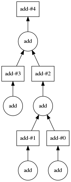
Dask has many many more features that what I have shown above and make a very compelling case to using it. I would recomend installing dask[complete] and some of the additional dependencies bokeh and graphviz. Make sure to check out the dashbaord.

XND

The next tool I would like to talk about is XND. XND is a library that is being created by the efforts of Quansight. As I understand it, XND is an attempt to make a numpy that has richer support for types, usable from multiple languages, and is broken into components that help dependent libraries on numpy such as pandas. Due to some of the shortcoming of numpy several libraries have implemented their own numerical libraries such as tensorflow, pytorch, and Theono. Their are plans to have numerical kernels for XND that can work with both CPUs and GPUs. This is done using an awesome package numba. I have provided a set of working notebooks that you can try out with mybinder at github.com/costrouc/xnd-notebooks.

Numba

Numba is a library for speeding up a subset of the python language that is compatible with GPUs and CPUs. In my opinion numba is a way to target heterogeneous architectures easily with python. It compiles python functions into an LLVM AST. I think that a large part of numba gained inspiration from how Julia handles LLVM. Here is an extremely simple example. You can do much much more complicated calculations.

import timeit

def foo():
    total = 0
    for i in range(100000):
        total += i
    return total

expression = """
foo()
"""

timer = timeit.Timer(expression, globals=globals())
n, total_time = timer.autorange()
print('time per run', total_time / n, 'seconds')
# time per run 0.006681793339998876 seconds

Now using numba. Obviously we all know that compiled code runs faster and it is possible that llvm compiled out all of the loop. Either way I hope this demos the basic usage.

from numba import jit

@jit
def foo():
    total = 0
    for i in range(100000):
        total += i
    return total
foo()

expression = """
foo()
"""

timer = timeit.Timer(expression, globals=globals())
n, total_time = timer.autorange()
print('time per run', total_time / n, 'seconds')
# time per run 9.659497299999203e-08 seconds

You can even inspect the llvm that is generated from the function.

from numba import jit

@jit
def foo():
    total = 0
    for i in range(100000):
        total += i
    return total
foo()

for key, value in foo.inspect_llvm().items():
    print(key, value)

() ; ModuleID = 'foo'
source_filename = "<string>"
target datalayout = "e-m:e-i64:64-f80:128-n8:16:32:64-S128"
target triple = "x86_64-unknown-linux-gnu"

@.const.foo = internal constant [4 x i8] c"foo\00"
@".const.Fatal error: missing _dynfunc.Closure" = internal constant [38 x i8] c"Fatal error: missing _dynfunc.Closure\00"
@PyExc_RuntimeError = external global i8
@".const.missing Environment" = internal constant [20 x i8] c"missing Environment\00"

; Function Attrs: norecurse nounwind
define i32 @"_ZN8__main__7foo$242E"(i64* noalias nocapture %retptr, { i8*, i32 }** noalias nocapture readnone %excinfo, i8* noalias nocapture readnone %env) local_unnamed_addr #0 {
entry:
  store i64 4999950000, i64* %retptr, align 8
  ret i32 0
}

define i8* @"_ZN7cpython8__main__7foo$242E"(i8* %py_closure, i8* %py_args, i8* nocapture readnone %py_kws) local_unnamed_addr {
entry:
  %.5 = tail call i32 (i8*, i8*, i64, i64, ...) @PyArg_UnpackTuple(i8* %py_args, i8* getelementptr inbounds ([4 x i8], [4 x i8]* @.const.foo, i64 0, i64 0), i64 0, i64 0)
  %.6 = icmp eq i32 %.5, 0
  br i1 %.6, label %entry.if, label %entry.endif, !prof !0

entry.if:                                         ; preds = %entry
  ret i8* null

entry.endif:                                      ; preds = %entry
  %.10 = icmp eq i8* %py_closure, null
  br i1 %.10, label %entry.endif.if, label %entry.endif.endif, !prof !0

entry.endif.if:                                   ; preds = %entry.endif
  %.12 = tail call i32 @puts(i8* getelementptr inbounds ([38 x i8], [38 x i8]* @".const.Fatal error: missing _dynfunc.Closure", i64 0, i64 0))
  unreachable

entry.endif.endif:                                ; preds = %entry.endif
  %.14 = ptrtoint i8* %py_closure to i64
  %.15 = add i64 %.14, 24
  %.17 = inttoptr i64 %.15 to { i8* }*
  %.181 = bitcast { i8* }* %.17 to i8**
  %.19 = load i8*, i8** %.181, align 8
  %.24 = icmp eq i8* %.19, null
  br i1 %.24, label %entry.endif.endif.if, label %entry.endif.endif.endif, !prof !0

entry.endif.endif.if:                             ; preds = %entry.endif.endif
  tail call void @PyErr_SetString(i8* nonnull @PyExc_RuntimeError, i8* getelementptr inbounds ([20 x i8], [20 x i8]* @".const.missing Environment", i64 0, i64 0))
  ret i8* null

entry.endif.endif.endif:                          ; preds = %entry.endif.endif
  %.46 = tail call i8* @PyLong_FromLongLong(i64 4999950000)
  ret i8* %.46
}

declare i32 @PyArg_UnpackTuple(i8*, i8*, i64, i64, ...) local_unnamed_addr

; Function Attrs: nounwind
declare i32 @puts(i8* nocapture readonly) local_unnamed_addr #1

declare void @PyErr_SetString(i8*, i8*) local_unnamed_addr

declare i8* @PyLong_FromLongLong(i64) local_unnamed_addr

; Function Attrs: nounwind
declare void @llvm.stackprotector(i8*, i8**) #1

attributes #0 = { norecurse nounwind }
attributes #1 = { nounwind }

!0 = !{!"branch_weights", i32 1, i32 99}

pymc3

PyMC3 is a package that has always fascinated me. While I do most of my machine learning tasks in scikit-learn, I really have an appreciation for bayesian statistics. The ability for carry the uncertainty with the measurement is a great tool to have. PyMC3 is powerful in that it has a domain specific language in python for representing your bayesian model. There were two talks given on PyMC3 during pycon. One investigated gerymandering in North Carolina while the other talk showed the power of gaussian processes. Gaussian processes have begun to be heavily used in hyperparameter tuning for neural networks. It allows for a "parameter free" approach to tuning your neural network (it in actuality an infinite parameter model). Here is a simple example of its usage many more examples can be seen in the documentation.

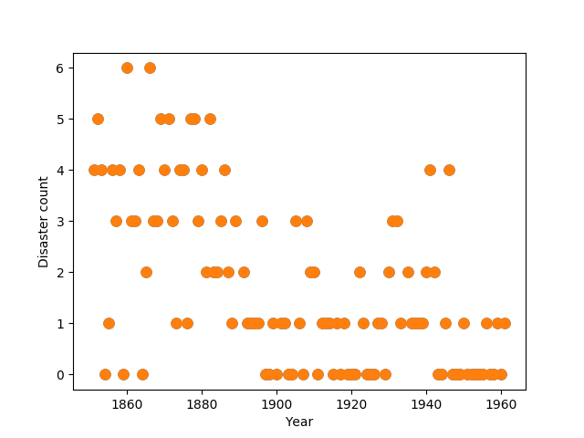
Consider the following time series of recorded coal mining disasters in the UK from 1851 to 1962 (Jarrett, 1979). The number of disasters is thought to have been affected by changes in safety regulations during this period. Unfortunately, we also have pair of years with missing data, identified as missing by a NumPy MaskedArray using -999 as the marker value.

import pymc3 as pm
print('Running on PyMC3 v{}'.format(pm.__version__))
# Running on PyMC3 v3.4.1

import numpy as np
import matplotlib.pyplot as plt

disaster_data = np.ma.masked_values([4, 5, 4, 0, 1, 4, 3, 4, 0, 6, 3, 3, 4, 0, 2, 6,
                            3, 3, 5, 4, 5, 3, 1, 4, 4, 1, 5, 5, 3, 4, 2, 5,
                            2, 2, 3, 4, 2, 1, 3, -999, 2, 1, 1, 1, 1, 3, 0, 0,
                            1, 0, 1, 1, 0, 0, 3, 1, 0, 3, 2, 2, 0, 1, 1, 1,
                            0, 1, 0, 1, 0, 0, 0, 2, 1, 0, 0, 0, 1, 1, 0, 2,
                            3, 3, 1, -999, 2, 1, 1, 1, 1, 2, 4, 2, 0, 0, 1, 4,
                            0, 0, 0, 1, 0, 0, 0, 0, 0, 1, 0, 0, 1, 0, 1], value=-999)
year = np.arange(1851, 1962)

plt.plot(year, disaster_data, 'o', markersize=8);
plt.ylabel("Disaster count")
plt.xlabel("Year");
filename = os.path.expanduser(os.path.join(image_dir, 'coal_mine.png'))
plt.savefig(filename)
_ = filename

$D\_t \sim \text{Pois}(r\_t), r\_t= \begin{cases} l, & \text{if} t \lt s \\ e, & \text{if } t \ge s \end{cases}$

$s \sim \text{Unif}(t\_l, t\_h)$

$e \sim \text{exp}(1)$

$l \sim \text{exp}(1)$

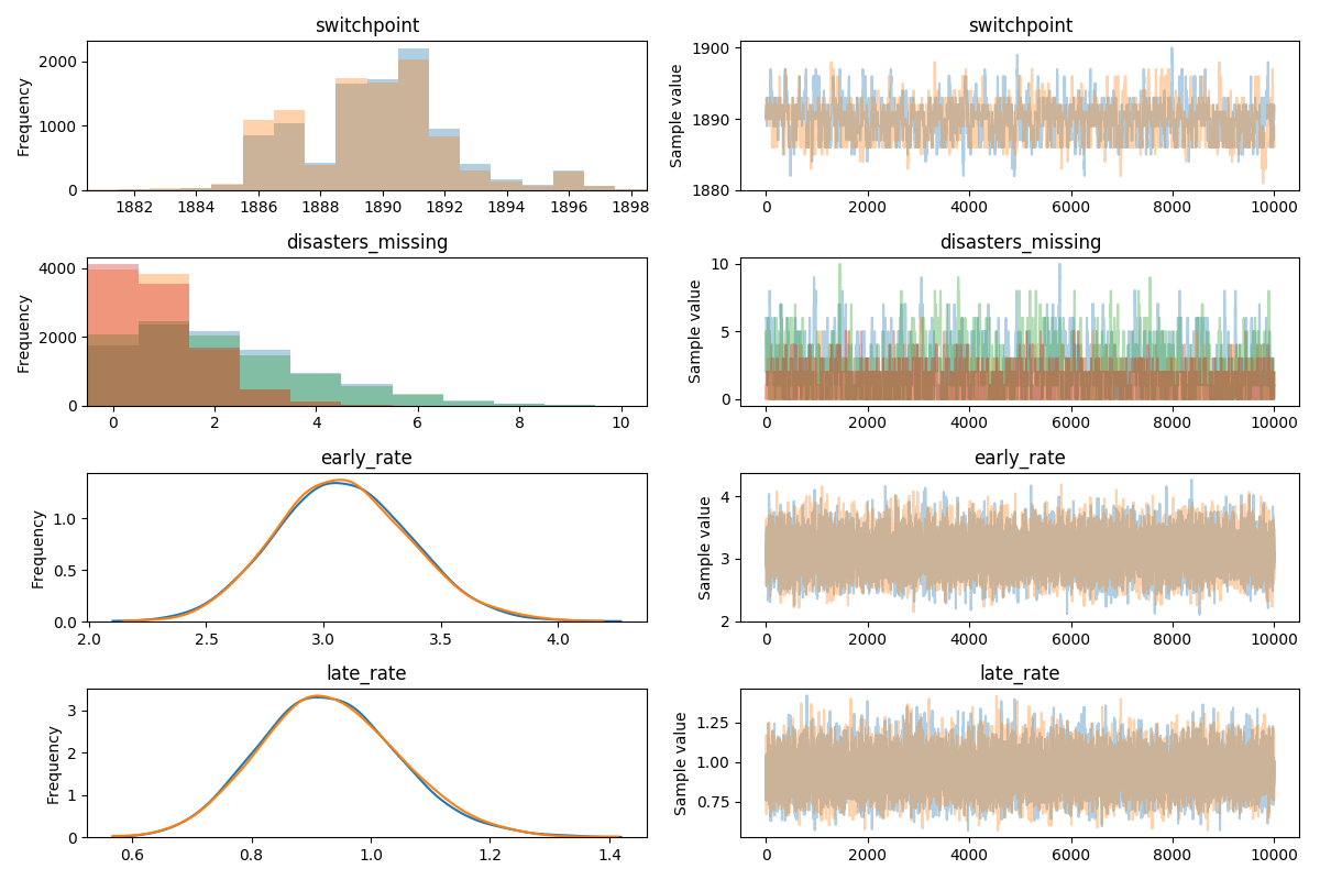
Lets define the model in code.

with pm.Model() as disaster_model:

    switchpoint = pm.DiscreteUniform('switchpoint', lower=year.min(), upper=year.max(), testval=1900)

    # Priors for pre- and post-switch rates number of disasters
    early_rate = pm.Exponential('early_rate', 1)
    late_rate = pm.Exponential('late_rate', 1)

    # Allocate appropriate Poisson rates to years before and after current
    rate = pm.math.switch(switchpoint >= year, early_rate, late_rate)

    disasters = pm.Poisson('disasters', rate, observed=disaster_data)
    trace = pm.sample(10000)

Sequential sampling (2 chains in 1 job)
CompoundStep
>CompoundStep
>>Metropolis: [disasters_missing]
>>Metropolis: [switchpoint]
>NUTS: [late_rate_log__, early_rate_log__]
100% 10500/10500 [00:18<00:00, 570.13it/s]
100% 10500/10500 [00:16<00:00, 651.36it/s]
The number of effective samples is smaller than 10% for some parameters.

pm.traceplot(trace)
filename = os.path.expanduser(os.path.join(image_dir, 'coal_mine_var_fit.png'))
plt.savefig(filename)
_ = filename

And that is a summary of my great learning experience at pycon. I want to thank everyone there for making it such an enjoyable conference!